[% INCLUDE header.us3
title = 'UltraScan III Equilibrium Time Estimator'
%]
Estimating Equilibrium Time
Whenever you are planning or designing an equilibrium experiment, the question
comes up of how long it takes to reach equilibrium at a certain speed. The
time it takes depends on several factors:
- The model of the solution will govern the experiment simulation. Use
the Model Editor to set the following
parameters:
- The diffusion coefficient. The smaller the diffusion coefficient,
the longer it will take to reach equilibrium, since the sample will
diffuse slower. Asymmetric and random coil molecules will take longer
to equilibrate than globular molecules with the same molecular
weight.
- The sedimentation coefficient. The larger the sedimentation
coefficient, the faster the molecule will equilibrate, provided the
diffusion coefficient stays constant, which is rarely the case. As
molecular weight and sedimentation coefficient increase, the diffusion
coefficient will generally decrease, which has the opposite
effect.
- The moluculate weight.
- The position inside the rotor. The further to the outside of the rotor
the sample is positioned, the faster the sample will equilibrate, since the
centrifugal force is larger at the outside.
- The column length. The longer the column (the more volume is loaded),
the longer it will take to equilibrate.
- Finally the rotor speed. The larger the rotorspeed, the faster the sample
will approach equilibrium.
- It also matters if the system is at chemical equilibrium, and if that
equilibrium can be established rapidly enough (on the time order of the
experiment). If a monomer-dimer equilibrium experiment takes a long time
to equilibrate (i.e., the equilibrium kinetics are not diffusion controlled),
then it may take substantially longer than predicted by this program.
THis program will only predict the experiment of a diffusion controlled
kinetics environment.
How to use this program:
When designing an equilibrium experiment, you should plan to acquire
equilibria at multiple speeds (4-5 speeds, ranging from
sigma=1 to sigma=5). Using the finite element simulator
programmed in this module, you can predict the time it takes to reach
equilibrium for all practical purposes, i.e., the change over time is less
than a certain tolerance value. You can then pre-program the speeds into
the XLA and are not required to check for equilibrium evertime before you
change to the next speed.
Note: Sigma is a measure of the curvature of the exponential. If it is
too small, the curvature is shallow and there is not enough information. If
it is too steep, most of the concentration points are going to be near
zero, drowned out by bad s/n ratios. The happy medium is between 1 < sigma
< 4, as far as equilibrium exponents are concerned. It's a convenient way
to parameterize curvature, which is a function of rotor speed and molecular
weight.
When simulating these times, you should simulate a molecule that is
sedimenting slightly slower than the actual molecule, perhaps by simulating
a system with a larger frictional ratio or larger axial ratio, and perhaps
a nonglobular model rather than a spherical model. While the equilibrium
times may be longer than needed, at least they won't be too short. In this
module you can change the parameters that influence the time it takes to
reach equilibrium.
Explanation for fields and buttons:
- Set / Change / Review Model
- Use thie pushbutton to bring up the Model Editor.
- Radius Settings
- Chose a predfined top and bottom radius settings with the Channel Type
radio buttons. Use the Custom button to manually define the radius settings.
- Rotorspeed Settings
- Select the appropriate radio button to enter the speeds in terms of
sigma (reduced molecular weight term:
(M * omega2 * (1 - vbar * rho))/ 2 * R * T) or by RPM.
- Low Speed: Select the first speed to be equilibrated
- High Speed:Select the last speed to be equilibrated
- Speed Steps: The total number of speeds to be simulated,
including the high and low speed. These will be linearly spaced
between the high and low speed.
- Current Speed List: All selected speeds will be listed here. This
field cannot be edited directly.
Note: All speeds will be adjusted to the nearest 100 rpm, so they can
be programmed in the XLA, which only allows 100 rpm steps.
- Simulation Settings
-
- Tolerance: This value is the tolerance setting that determines if
a scan has reached equilibrium. Successive scans are subtracted from
each other and the root mean square of the differences are calulated.
If the difference is less or equal to this tolerance value, the
program will consider the speed equilibrated and automatically
proceed to the next speed. For a 3 mm column with 0.001 cm resolution
the accuracy of the computer allows about 1.0x10⁻⁵ for the
smallest practical tolerance (noise-free data).
- Time Increment (min): This is the time between successive scans.
The larger the time difference, the coarser is the time
determineation, but the more reliable is the time estimation. A good
default setting is 15 minutes, to be used with a 5 x 10⁻⁴
tolerance setting.
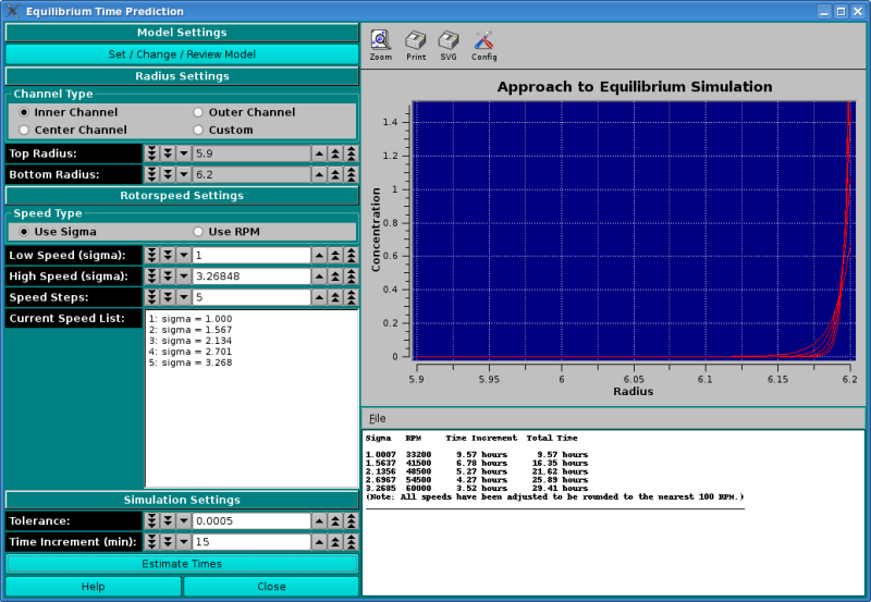
- Estimate Times Pushbutton
- This function runs the simulation and populates the graph and the
text window. The text can be saved with the File dropdown list
abive the text window.
[% INCLUDE footer.us3 %]
 Manual